Chirp sounder measurements with KiwiSDRs (1)

The plots below show measurements of the chirp sounders from Cyprus (RAF Aktrotiri). There are two chirps (100kHz/sec) separated by 5 seconds and repeating each 5 minutes. In G3PLX notation they are called 300:240 and 300:245. 

Using GNSS timestamped IQ samples from the KiwiSDR @IU8CRI, tuned to 13,200 kHz, a pair of chirps was analyzed in terms of instantaneous frequency and of propagation time delays obtained from the FFT of the de-chirped signals.

Top: instantaneous frequency; bottom: propagation time delay obtained form the FFT of the de-chirped signal

In this earlier blog post a time offset of about δt=0.3±0.03 msec w.r.t. start time at the beginning of a given UTC second of the chirp signals from Cyprus was found in the chirp monitoring data from the U Twente WebSDR. This offset is also found in the KiwiSDR measurements, i.e., without applying this offset, the first peak in the propagation time delays would be below the equivalent time of propagation along the great-circle distance at the speed of light.

It would be very interesting to implement a more systematic monitoring of chirp sounders using KiwiSDRs.

KiwiSDR IQ data streams with >20.25 kHz bandwidth (2)

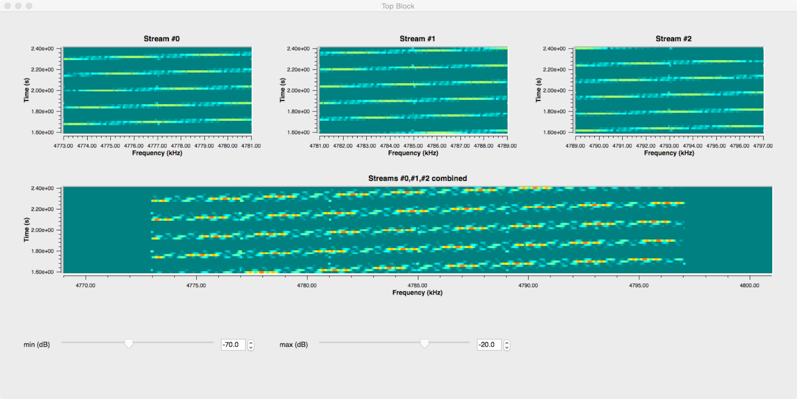
This is a follow-up on the last blog post. Since then a compensation for the roll-off of the CIC filters in the KiwiSDR FPGA has been implemented in v2.162.

The plot below shows the correction w.r.t. normalized frequency for the 12kHz (20.25kHz) modes in blue (magenta). It is interesting that the main component is in both cases sinc(f)^-5 and that the softening of the correction near f=0.5 can be modeled by an exponential function.

KiwiSDR CIC filter compensation

Another improvement w.r.t. before is to use ±4kHz out of the ±6kHz IQ bandwidth in order to avoid alias images from frequencies below and from above, so the GNURadio flow graph looks now like this:

GNURadio flow graph

This flow graph and the code for the KiwiSDR IQ wav file sources and for the stream align block can be found on GitHub (gr-kiwisdr).

In order to verify that the combination of three IQ data streams@8kHz each to an IQ datastream @32kHz does indeed work, two signals were recorded and processed with the above flow graph:

1.  OTHR signal from Cyprus
   
   

   

   Cyprus OTHR on 14370 kHz @IS0KYB

   As is well-known this signal has a bandwidth of 20kHz and uses a FMCW waveform repeating each 0.02 seconds. When plotting the instantaneous frequency vs. time the FMCW sweeps can be see to be perfectly continuous, i.e., both the alignment of the IQ data streams and the PFB synchronizer work as expected.

   

   Cyprus OTHR on 14370 kHz @IS0KYB

   
   
2. CODAR WCNA
   
   The two plots below show a local CODAR signal recorded on a KiwiSDR in Newport, OR. Also in this case the frequency sweeps can be nicely seen. However it is not clear if the second component in the instantaneous frequency having negative slope is due to interference or due to aliasing in the KiwiSDR downconversion processing.
   
   

   

   Local CODAR signal on 4875 kHz @Newport, OR

   

   Local CODAR signal on 4875 kHz @Newport, OR

The IQ streams used above were recorded using kiwirecorder.py with commands similar to the  following:

./kiwirecorder.py -s sibamanna.duckdns.org,sibamanna.duckdns.org,sibamanna.duckdns.org -p 8073 -f 14362,14370,14378 -m iq -g 55 -w -L -4000 -H +4000 --log-level=info --dt-sec=60 --station=IS0KYB

KiwiSDR IQ data streams with >20.25 kHz bandwidth

Recently I got to implement a way of recording data from KiwiSDRs at more than 12 kHz (or 20.25 kHz) by combining streams of IQ data using a polyphase filter bank (PFB) synthesizer. Luckily the two most complicated blocks, the PFB synthesizer and delay blocks, are already available in GNURadio.

What was missing was a block reading KiwiSDR IQ data with GNSS timestamps and a block determining the delays of between the different IQ sources. As all of these come from the same KiwiSDR running the same ADC clock, the offsets are multiples of samples.

For testing I started with a CODAR signal centered around 4820kHz using the AB1BD KiwiSDR. IQ wav files with GNSS timestamps were recorded on 4808, 4820, 4832 kHz, each with 12kHz bandwidth. In order to avoid wrapping around one of the inputs, a PFB synthesizer with 4 channels and 3 inputs was used:

GNURadio flowgraph

The screenshot below shows the three input signals samples with 12kHz and the reconstructed signal @48kHz:

• Gain vs. frequency for the input signals is not flat. This is a known feature of the KiwiSDR FPGA code (missing CIC filter compensation filters). As a consequence there are dips in the combined spectrum
• Nevertheless the CODAR sweeps can be seen to be continuous in the combined waterfall display

Top: waterfall diagrams for three IQ streams @12kHz; bottom: combined IQ stream @48kHz

Another test is to look at the instantaneous frequency in the combined IQ data stream @48kHz which looks fine:

Instantaneous frequency vs. time for the combined IQ data @48kHz

Obviously this has more applications than CODAR data analysis, as it opens up the possibility to analyze signals with up to 36kHz bandwidths. When a PFB synthesizer with 6 channels is used, up to 5 KiwiSDR IQ streams can be combined which enlarges the bandwidth to 60 kHz. Instead of using prerecorded wav files, the KiwiSDR GNURadio block can be used to combine streams of IQ samples in realtime.

The code for this will be made available as part of gr-kiwisdr after some cleanup.

KiwiSDR GNURadio block

A first version of a GNURadio interface gr-kiwisdr for the KiwiSDR is available on GitHub. It consists of a GNURadio source block which connects to a given KiwiSDR and provides a stream of IQ samples.

At this moment gr-kiwisdr is not yet complete but fully working. Missing items include support for

• other modes than IQ mode (not sure if this is really useful)
• user login and non-default AGC settings
• stream tags containing GNSS timestamps

For connecting to the KiwiSDR websocket server boost.beast is used. Because the available boost versions, e.g., on Ubuntu, are fairly old and boost.beast is a recent addition to boost, gr-kiwisdr contains git submodules for boost.asio and boost.beast (both are header-only libraries).

Any feed-back is very much welcome.
As an example, the preamble cross-correlation of a STANAG 4285 signal is shown below. The two secondary cross-correlation peaks are there because the 80-symbol long STANAG 4285 preamble consists of repetitions of a 31-bit long pseudo-random sequence generated by a LFSR.

Real-time preamble cross-correlation for a STANAG4285 signal.

GRC flow-graph for the plot shown above.

KiwiSDR GNSS position solutions using an extended Kalman filter

This is an update to this blog post, see also https://github.com/jks-prv/Beagle_SDR_GPS/issues/147. References for using Kalman filters for GNSS positioning are, e.g., DST-Group-TR-3260.pdf and these proceedings from ION GPSGNSS 2003.

The plots below show time series of variations in ECEF X,Y,Z coordinates, the oscillator correction, and the number of available satellites.

SPP - single point position; EFK - extended Kalman filter

The process noise covariances are set to 5e-5 for the X,Y,Z coordinates (KiwiSDRs are not expected to move) and the covariances for the time and the oscillator correction are build from Allan variance parameters as described in a497248. It would be interesting to measure the Allan variance of the used oscillator.

The advantages of using an extended Kalman filter include:

• Once a position solution has been obtained, the Kalman filter can be updated with fewer than four satellites: this will improve the availability of those KiwiSDRs with poor GNSS reception for TDoA work.
• The residuals per link in the Kalman filter update are used to exclude satellites with bad time measurements.
• Large deviations from the nominal position due to bad satellite geometries are avoided.

New version of TDoA code available

A version of the 1st idea mentioned in the last blog post is now implemented in the latest version of the TDoA code and thanks to John it is available as an option in the KiwiSDR TDoA service.

The changes in the new TDoA algorithm are the following:

(1) Sanity checks on the recorded IQ wav files

Instead of aborting processing when a single file is found to be bad, stations are now excluded. If more than 1 good station is left, the processing proceeds without the excluded stations. The following checks are performed:

• check for recent GNSS position fixes
• validity check on then GNSS timestamps
• check if |IQ|!=0
• check if the overlap of all wav files is long enough (>10 sec)

(2) Finding clusters in the cross-correlation peaks

For a given pair of stations, peaks in the cross-correlations are found as before. Then these peaks are assembles into up to four clusters using an adaptive clusterization algorithm. It starts by assuming that there are four clusters. If the four clusters are not valid, the algorithm starts again, this time assuming that there are three clusters. When all clusters are valid the algorithm terminates.

The used clusterization algorithm is iterative:

• It starts by assuming that there are N clusters and puts N+1 boundaries b_i at equidistant places between the minimum and maximum time of the cross correlation peaks.
• Then it recomputes the boundaries as follows: Let t_i,i+1 be the average of the mean of the cross correlation peaks between b_i and b_i+1. The boundaries are iteratively updated as b_i=(t_i-1,i+t_i,i+1)/2 until they become constant.
• A cluster is called valid if the distribution of entries in it is not compatible with a random distribution.
• If all clusters are valid or if there is only one cluster (N=1) then the clusterization algorithm terminates.

(3) Selection of those clusters which optimally fulfill the consistency equations

• If there are three stations, cross-correlation times of the same signal fulfill (12)-(13)-(23)=0.
• When there are four stations, there are more of these consistency equations, e.g., (12)-(14)-(24)=0, (23)-(24)-(34)=0 etc.
• For all combinations of clusters all consistency equation are evaluated. Each equation provides the deviation from 0 in terms of number of sigmas (nsigma) using the mean and RMS of the clusters.
• In the end the combination of clusters is selected which for all consistency equations results in the smallest nsigma
• If the nsigma value in any given equation is greater than 3, stations are iteratively excluded until 3 stations are left. The combination of excluded stations which brings max(nsigma) below 3 is not used later on for making the TDoA maps.

New ideas for TDoA multi-lateration

(1) Finding the common propagation mode

Let's consider the case of three receivers receiving the same signal.

• Each receiver receives the signal at times t₁, t₂, t₃.
• The cross-correlations produce time differences Δt_1,2, Δt_1,3, Δt_2,3.
• Trivially, Δt_1,2 = Δt_1,3 - Δt_2,3 (and cyclically) (*)

This situation is illustrated in the plot below.

Common propagation mode

As a second step let's consider the situation when one of the three receivers receives the common signal via two propagation paths, and the cross-correlations to the signals received at the two other receivers have approximately the same magnitude.

Currently the TDoA software performs for each cross-correlation a clustering algorithm, and in the situation shown in the plot below it may well be that the following time differences are obtained: Δt_1,2 = -50, Δt_1,3 = -100, Δt_2,3 = -140. Note that these do not fulfill the identity (*).

Two propagation modes for one receiver

As a consequence, a trivial stage of pre-processing is given by selecting those cross-correlation peaks which are consistent according to (*).

Update 9/22/2018

(2) Using constraints (number of degrees of freedom)

Now let us count the number of degrees of freedom for the case of N receivers receiving the same signal: there are

• 2 unknowns, (lat,lon), for the most likely position
• N unknown virtual heights of which only (N-1) are observable in the time differences (adding a common time offset does not change Δt_i,j)
• N(N-1)/2 hyperbolæ (=constraints)

Note that instead of virtual heights we might as well add time offsets δt_j  to the time differences, Δt_i,j+δt_j, j≠1, and in this way become agnostic w.r.t. the specifics of ionospheric propagation.

As a summary there are N+1 unknowns and N(N-1)/2 constraints:

#receivers	#unknowns	#constraints	#constraints-#unknowns
3	2(pos)+2(δtj, j≠1)	3 hyperbolæ	-1
4	2(pos)+3(δtj, j≠1)	6 hyperbolæ	1
N	2(pos)+(N-1)(δtj, j≠1)	N(N-1)/2 hyperbolæ	N(N-1)/2-N-1

So for 3 receivers there is a 1-dimensional family of solutions while for N≥4 receivers the system of equations is overdetermined.  This sounds good enough to make me suspicious if it is indeed true.

---

It will be interesting to try these ideas on real data obtained from KiwiSDRs. If anyone spots an error in the logic above please do let me know.

---

When using N stations there are N-1 independent measurements contained in the time differences δt_ij, j>i. Two of these are needed to determine the likely position, so N-3 out of the N-1 δt_i, i≠1, can be found:

#receivers	#unknowns	#measurements	#fixed/total δtj
3	2(pos)+2(δtj, j≠1)	2 time differences	0/2
4	2(pos)+3(δtj, j≠1)	3 time differences	1/3
5	2(pos)+4(δtj, j≠1)	4 time differences	2/4
6	2(pos)+5(δtj, j≠1)	5 time differences	3/5
N	2(pos)+(N-1)(δtj, j≠1)	(N-1) time differences	(N-3)/(N-1)