Measuring oblique ionograms using KiwiSDRs (1)

Oblique ionogram obtained from a KiwiSDR using GNSS timestamps

How it is done

The receive bandwidth of KiwiSDRs is limited to 12 kHz (20.25 kHz in 3 user channel configuration). In order to synchronously tune to a chirp sounder GNSS-based timestamps are used:

• For the current GNSS timestamp T0 tune the KiwiSDR to the frequency on which the chirp is expected at a time T0+DT.
• Record 10240 IQ samples, corresponding to 20 512-sample long buffers
• Repeat

Timing diagram

In this way, the chirp is always seen at a specific offset. Note that the tuning frequencies are different for each different complete chirp sweep because the KiwiSDR sampling rate is not GNSS-disciplined (the GNSS timestamps are exact).

abs(IQ) vs. frequency

For a chirp rate of 100 kHz/s and sampling rate 12 kHz, the frequency steps are ~85.33 kHz and the group delay resolution is 25 km.

The time offset DT, which depends on the delay between issuing a frequency change command and its effect, is measured at the beginning. It depends on internal KiwiSDR delays and on the network delay. If the KiwiSDR is on a local network this delay is about 2 buffers long, for KiwiSDRs on the internet delays between 8 and 10 buffers were seen.  

KiwiSDR gets CIC compensating filters

In an upcoming update, KiwiSDR's will get proper CIC compensating filters.

How is down-conversion done in the KiwiSDR?

The ADC runs at 66.66666 MHz, and CIC filters are used to down-convert to either 12 or 20.25 kHz. I recommend reading the original paper by Hogenauer which explains how to choose the bit widths of each filter stage in an optimal way.

Down-conversion from 66.66666 MHz to 12kHz (20.25kHz) is done in two steps; for the 12 kHz mode a 1st CIC filter is used to decimate by a factor of 926 to ~72 kHz; this is followed by a 2nd CIC which decimates by a factor of 6 to ~12 kHz.

The problem with CIC filters

CIC filters are optimal in the sense that they do use only addition and subtraction, as opposed to generic FIR filters, and therefore can be efficiently implemented in an FPGA. However, they are not perfect: 

• All signals outside the fundamental domain (+- 6kHz in this case, green dashed lines in the graph below) are mirrored/reflected into it.
• The filter curve of CIC filters is not flat, i.e., there is filter roll-off.

CIC filter response.

Enter CIC compensating filters

Both of these issues are improved by using a CIC compensating filter: instead of using the 2nd CIC filter for down-sampling to 12kHz, it is replaced with another CIC filter which down-samples to 24kHz, followed by a low-pass FIR filter and a final 2:1 down-sampling. The FIR filter makes sure everything out of +-6kHz is suppressed and that the CIC filter roll-off is compensated for. See AN455 for details.

CIC compensating filter with 64 taps for the 12 kHz mode.

CIC compensating filter performance

Using the built-in KiwiSDR signal generator the performance of the CIC+CIC compensating filter can be measured:

• Signal generator is set to sweep from 10 MHz to 10.012 MHz
• IQ mode recording
• Manual AGC
• Any other CIC compensation used previously turned off

Left: waterfall diagram: time vs. frequency; right: blue - signal, red - background.

• The residual CIC filter roll-off from the 1st CIC filter is < 0.2 dB (only the roll-off of the 2nd CIC filter is compensated for)
• Mirror signals are smaller than approximately -50 dB

HF Over-the-horizon radar processing using GNSS timestamped KiwiSDR IQ samples

OTHR parameters: 

• Chirp repetition time Δt=20 msec
• frequency slope=1 MHz/sec.

Its bandwidth is 20 kHz which fits nicely into the 20.25 kHz bandwidth of KiwiSDRs in 3-ch mode. 

Instantaneous frequency vs. mod(gpssec, 20 msec)

In the following we use GNSS-timestamped IQ samples for performing bi-static radar processing:

• Dechirping and framing into 20 msec long GPS-time-aligned frames
• interpolation in each frame (512 samples/frame)
• compute the 1st FFT along rows -> relative range
• compute the 2nd FFT  along columns on the result from the previous steps -> relative Doppler shift

Shown below are maps with relative Doppler frequency vs. relative range for 30 1-minute long periods, i.e., averaged over 1500 chirps each:

• the main signal comes at two different Doppler shifts and two different ranges, corresponding to two different ionospheric propagation paths.
• The pattern for the main signal can be found in several other places as well: this should correspond to reflections off some targets where the reflected signal then propagates with similar paths than the main component.
• It is interesting that besides the main component there are several instances of another pattern present, having two different Doppler shifts and ranges.
• It might also be that the secondary peaks are artifacts created by the signal processing.

Animation showing relative Doppler frequency vs. relative range.

AM modulation index

This is not the most exciting topic, but on the KiwiSDR forum there were repeated questions on how to measure the AM modulation index.

The best reference which I have found for that is an report from the ITU, R-REP-BS.2433-2018-PDF-E, where the "RMS modulation depth", i.e., the RMS ratio of side-bands and the carrier is being used as a proxy for the modulation index.

GNURadio flowgraph for measuring AM RMS modulation depth 

First, synchronous AM demodulation is performed using a PLL which locks onto the carrier. Then the RMS power in the carrier and in the side-bands is computed and their ratio is formed. Smoothed versions of this variable are shown a number and as a histogram. Note that the "RMS AM modulation depth" block consists of just a few lines of python.

The grayed out, i.e., disabled portions of this flowgraph were used to verify that the normalization is correct.

For the BBC transmitter on 198 kHz, the RMS modulation depth was found to be about 12% at the time of measurement which is consistent with the value quoted in the ITU report mentioned above. However, this number can vary by a factor of 1.5 or more (9-18%) depending on whether the program consists of speech or of music at the time of measurement. Furthermore,  the measured modulation depth indicates that dynamic carrier suppression is being used, see again the ITU report for details.

AM RMS modulation depth for BBC on 198 kHz

HF TDoA multilateration (2)

This is an update to the last blog post where propagation delays from VOACAP are used in addition to great-circle-derived propagation delays.

As VOACAP provides a number of propagation modes (MODE=25) the mode which is most close to the measured time difference is used.

Note that the findings in the plots below might accidentally: when there are enough closely-spaced delays available it is quite likely to match the data.

Nevertheless it can be seen that large deviation from the hypothesis of ground-wave propagation along great-circle paths are due to different reflection heights, i.e.,  1E-1F2, 2F1-1F2, etc: at a given time, a number of different propagation paths are available, and for different combinations of receivers, different propagation modes are in fact observed.

Comparison of measured time delay differences with differences based on ground-wave propagation along great-circle paths and differences based on VOACAP predictions.

Comparison of measured time delay differences with differences based on ground-wave propagation along great-circle paths and differences based on VOACAP predictions.

HF TDoA multilateration (1)

This blog post contains an analysis of TDoA multilateration applied to signal on 13413.4 kHz using a number of KiwiSDRs located in Europe.

For now the assumption used for making the KiwiSDR TDoA maps is that signals propagate with speed of light along the ground. Here we compare the measured delay differences with the ones obtained from this assumption.

All plots shown in this blog post are generated using octave/matlab .mat files available when using the updated KiwiSDR TDoA algorithm.

The cross-correlations for all combinations of used KiwiSDRs, normalized to have their maximum at unity, are shown below.

cross-correlations

Differences between the measured values and the ones obtained from great-circle-derived time delay differences are due to ionospheric propagation. As expected, the ionospheric effects tend to cancel for pairs of KiwiSDRs which are at about the same distance to the transmitter:

Comparison of  measured with great-circle time differences

The following scatter plot shows the effect of ionospheric propagation w.r.t. great-circle propagation. It will be very interesting to re-do this analysis using propagation delays e.g. from VOACAP instead of assuming propagation along great-circles at ground level.

Scatter plot for time differences

Slightly earlier the plots looked like this:

cross-correlations

Comparison of  measured with great-circle time differences

Scatter plot for time differences

Some HF radar signals

7500 kHz

A number of similar HF radar signals have recently been observed on KiwiSDRs located in Europe on different frequencies.

The pulse repetition rate is 40 Hz (25 ms/pulse).

abs(IQ)

Each pulse consists of a linear chirp and of a pause.

FM demodulation

KiwiSDR TDoA multilateration indicates that these signals come from somewhere in Russia.

KiwiSDR TDoA multilateration

Bursts of what seem to be linear FM chirps have been observed on different frequencies around 8050±~50 kHz.

6390 kHz

Like the signal on 7500 kHz the pulse repetition rate is 40 Hz. However the duty cycle is smaller.

abs(IQ)

FM demodulation

8050 kHz

For this signal, the pulse repetition rate is 96 Hz.

abs(IQ)

Each pulse consists likely of a linear chirp. The spikes in the instantaneous frequency seen below are probably cause by HF propagation effects. Note that these radar-like signals are narrow-band (±1kHz variation in instantaneous frequency, only)

FM demodulation

KiwiSDR TDoA multilateration indicates a position somewhere in the Atlantic Ocean (compatible with the Azores).

KiwiSDR TDoA multilateration

DGPS TDoA

Recently, some people have observed a DPGS signal on 318 kHz. Existing software displays its location as Shepelevskiy (Leningrad Oblast) ; however KiwiSDR TDoA shows a different likely location.

318 kHz DGPS

Chirp sounder measurements with KiwiSDRs (2)

Using the recent work on KiwiSDR waterfall recording (see kiwiclient/kiwiwfrecorder.py) it becomes possible to search for chirp sounder signals in KiwiSDR waterfall data, continuing the topic from this post.

kiwiwfrecorder.py connects both to the 'SND' and the 'W/F' websocket streams. The 'W/F' stream contains sequence numbers for each waterfall line which are used to synchronize the waterfall to the audio data. These sequence numbers can also be used to attach to each waterfall line a corresponding GNSS time tag obtained from the 'SND' stream. As the waterfall data can arrive before or after the audio data, both are combined in a third thread using python Queues for thread-safe communication.

About half an hour of waterfall data was recorded on the AB1LD KiwiSDR using the highest KiwiSDR waterfall speed which turns out to provide waterfall data about for each SND frame, i.e, each 512/12000 seconds. Thanks to the owner for setting up this KiwiSDR and allowing unrestricted access!.

Then the recorded waterfall data (saved in a .npy formatted file) was rebinned in time to 1024/12000 second bins and exported as a .png file. Switching from python to octave, a search for chirp sounders was performed for chirp rates from 80  kHz/s to 130 kHz/sec in steps of 1 kHz/sec: for each chirp rate and for each start time the content of the waterfall bins was summed up along the corresponding line (Hough transform).

Two chirp sounders were found, each having a repetition rate of 720 seconds (12 minutes) with chirp rates of 82 kHz/sec and 100 kHz/sec, respectively. It might be interesting that this list of chirp sounders contains entries for three chirps sounders with 720 second periods located in Norfolk, VA, Kingsville, TX, and in Puerto Rico.

The plots below show zoomed waterfall diagrams around the chirps and on the bottom panel the result of the chirp search, i.e, the sums of waterfall bins along lines with a given slope.

1^st chirp sounder detected using the AB1LD KiwiSDR

2^nd chirp sounder detected using the AB1LD KiwiSDD

Talk on KiwiSDR TDoA is available on YouTube

This is just a short note that my recent talk on KiwiSDR TDoA at the Software Defined Radio Academy 2019, which took place during the German Ham Convention in Friedrichshafen, Germany, is now available on YouTube.

For other talks from this meeting see http://youtube.sdra.io/.

KiwiSDR IQ data streams with >20.25 kHz bandwidth (5)

By now, gr-kiwisdr can coherently combine between 2 and 6 IQ data streams recorded from the same KiwiSDR.

Following an idea by WA2ZKD, the following test was made with DRM signals: three data streams were recorded, one centered on the DRM signal on 15120 kHz and two more centered on 15112.5 kHz and on 15127.5 kHz which were then coherently combined into a signal data stream. The GNURadio display is shown below:

Coherent combination of two IQ data streams using gr-kiwisdr.

Both, the WAV file centered on 15120 kHz, and the combined WAV file were successfully decoded by DREAM:

DREAM display

The SNR is comparable for both files, taking into account that it fluctuates by about ±0.5 dB:

DREAM waterfall display for the combined WAV file.

DREAM waterfall display for the WAV file recorded on the center frequency.

Only one slight difference was found in the SNR per carrier display: although the SNR per carrier is fluctuating quite a lot, for the combined WAV file there is a dip around the center which is not there for the WAV file recorded on the center frequency:

DREAM SNR per carrier display display for the combined WAV file.

DREAM SNR per carrier display for the WAV file recorded on the center frequency.

KiwiSDR IQ data streams with >20.25 kHz bandwidth (4)

This is a follow-up to this blog post.

The figure below summarizes how three IQ data streams with equal frequency offsets Δf are combined into a single IQ data stream with sampling frequency 4Δf:

Coherent combination of three KiwiSDR IQ streams

Note that the center frequencies are set to exact values, using GNSS timestamps to correct the local KiwiSDR oscillator, while the sampling frequencies of the IQ data streams are derived from the local KiwiSDR oscillator and are not exact. As a consequence the three IQ data streams are not coherent.

The three IQ data streams can be made coherent by 1) correcting for the frequency offsets and 2) aligning the relative phases.

1) Correcting for the frequency offset 

One way of describing this correction is by comparing a signal in stream#1 with frequency ΔF/2  and another signal in stream#2 with frequency -ΔF/2, taking into account that there are two different sampling rates: the true (GNSS aligned) sampling rate F_s and the sampling rate according to the state of the local KiwiSDR oscillator, F′_s :
         z₁(n) = exp{2πinΔF/2F′_s}
         z₂(n) = exp{2πinΔF/F_s - 2πinΔF/2F′_s} .
The beat offset signal is given by
         z₁^*(n) z₂(n) = exp{2πinΔF(1/F_s - 1/F′_s)} ,
and is used to correct for the frequency offset, where F′_s is determined from the GNSS time tags in the KiwiSDR IQ streams.

2) Relative phase alignment 

Having corrected the frequency offsets, we are left with constant relative phase differences, Δϕ(0,1) and Δϕ(1,2). These global phase offsets are estimated by cross-correlating the overlapping parts of the spectra, indicated in yellow in the figure above. GNURadio makes it easy to do this, using a combination of freq_xlating_ccf and conjugate__cc and a simple block which estimates the phase difference between two vectors of IQ samples.

Because the overlaps between IQ streams are needed to estimate the phase offsets, recordings with kiwirecorder.py should use the full available bandwidth.

The method described above has been implemented using GNURadio and is available as part of gr-kiwisdr. Please note that this is work in progress and might need further improvements.

As can be seen in the updated GRC flowgraph below, IQ stream sample alignment, the correction for coherence, and the PFB synthesizer were combined into a single GNURadio block, called coh_stream_synth. In addition, exp{iΔϕ(0,1)} and exp{iΔϕ(1,2)} are shown in a constellation diagram display in order to monitor phase coherence (=stable relative phases).

GRC flowgraph

Using the GNURadio PFB synthesizer with 2× oversampling (twox=True), edge effects at the boundaries between IQ data streams are avoided:

Coherent combination of three IQ streams @12 kHz into a single IQ stream @32 kHz.

Chirp sounder measurements with KiwiSDRs (1)

The plots below show measurements of the chirp sounders from Cyprus (RAF Aktrotiri). There are two chirps (100kHz/sec) separated by 5 seconds and repeating each 5 minutes. In G3PLX notation they are called 300:240 and 300:245. 

Using GNSS timestamped IQ samples from the KiwiSDR @IU8CRI, tuned to 13,200 kHz, a pair of chirps was analyzed in terms of instantaneous frequency and of propagation time delays obtained from the FFT of the de-chirped signals.

Top: instantaneous frequency; bottom: propagation time delay obtained form the FFT of the de-chirped signal

In this earlier blog post a time offset of about δt=0.3±0.03 msec w.r.t. start time at the beginning of a given UTC second of the chirp signals from Cyprus was found in the chirp monitoring data from the U Twente WebSDR. This offset is also found in the KiwiSDR measurements, i.e., without applying this offset, the first peak in the propagation time delays would be below the equivalent time of propagation along the great-circle distance at the speed of light.

It would be very interesting to implement a more systematic monitoring of chirp sounders using KiwiSDRs.

KiwiSDR IQ data streams with >20.25 kHz bandwidth (2)

This is a follow-up on the last blog post. Since then a compensation for the roll-off of the CIC filters in the KiwiSDR FPGA has been implemented in v2.162.

The plot below shows the correction w.r.t. normalized frequency for the 12kHz (20.25kHz) modes in blue (magenta). It is interesting that the main component is in both cases sinc(f)^-5 and that the softening of the correction near f=0.5 can be modeled by an exponential function.

KiwiSDR CIC filter compensation

Another improvement w.r.t. before is to use ±4kHz out of the ±6kHz IQ bandwidth in order to avoid alias images from frequencies below and from above, so the GNURadio flow graph looks now like this:

GNURadio flow graph

This flow graph and the code for the KiwiSDR IQ wav file sources and for the stream align block can be found on GitHub (gr-kiwisdr).

In order to verify that the combination of three IQ data streams@8kHz each to an IQ datastream @32kHz does indeed work, two signals were recorded and processed with the above flow graph:

1.  OTHR signal from Cyprus
   
   

   

   Cyprus OTHR on 14370 kHz @IS0KYB

   As is well-known this signal has a bandwidth of 20kHz and uses a FMCW waveform repeating each 0.02 seconds. When plotting the instantaneous frequency vs. time the FMCW sweeps can be see to be perfectly continuous, i.e., both the alignment of the IQ data streams and the PFB synchronizer work as expected.

   

   Cyprus OTHR on 14370 kHz @IS0KYB

   
   
2. CODAR WCNA
   
   The two plots below show a local CODAR signal recorded on a KiwiSDR in Newport, OR. Also in this case the frequency sweeps can be nicely seen. However it is not clear if the second component in the instantaneous frequency having negative slope is due to interference or due to aliasing in the KiwiSDR downconversion processing.
   
   

   

   Local CODAR signal on 4875 kHz @Newport, OR

   

   Local CODAR signal on 4875 kHz @Newport, OR

The IQ streams used above were recorded using kiwirecorder.py with commands similar to the  following:

./kiwirecorder.py -s sibamanna.duckdns.org,sibamanna.duckdns.org,sibamanna.duckdns.org -p 8073 -f 14362,14370,14378 -m iq -g 55 -w -L -4000 -H +4000 --log-level=info --dt-sec=60 --station=IS0KYB

KiwiSDR IQ data streams with >20.25 kHz bandwidth

Recently I got to implement a way of recording data from KiwiSDRs at more than 12 kHz (or 20.25 kHz) by combining streams of IQ data using a polyphase filter bank (PFB) synthesizer. Luckily the two most complicated blocks, the PFB synthesizer and delay blocks, are already available in GNURadio.

What was missing was a block reading KiwiSDR IQ data with GNSS timestamps and a block determining the delays of between the different IQ sources. As all of these come from the same KiwiSDR running the same ADC clock, the offsets are multiples of samples.

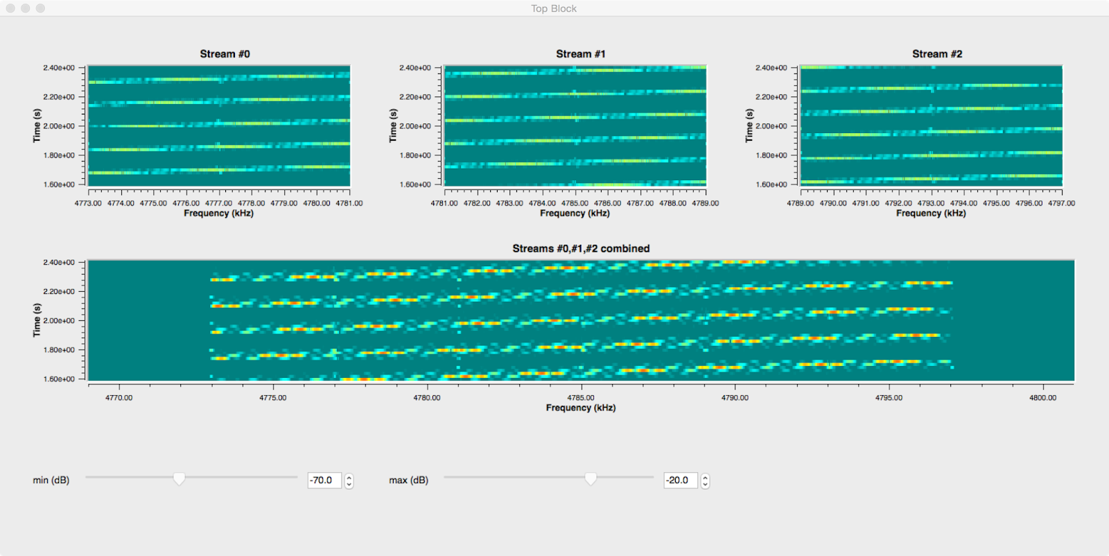
For testing I started with a CODAR signal centered around 4820kHz using the AB1BD KiwiSDR. IQ wav files with GNSS timestamps were recorded on 4808, 4820, 4832 kHz, each with 12kHz bandwidth. In order to avoid wrapping around one of the inputs, a PFB synthesizer with 4 channels and 3 inputs was used:

GNURadio flowgraph

The screenshot below shows the three input signals samples with 12kHz and the reconstructed signal @48kHz:

• Gain vs. frequency for the input signals is not flat. This is a known feature of the KiwiSDR FPGA code (missing CIC filter compensation filters). As a consequence there are dips in the combined spectrum
• Nevertheless the CODAR sweeps can be seen to be continuous in the combined waterfall display

Top: waterfall diagrams for three IQ streams @12kHz; bottom: combined IQ stream @48kHz

Another test is to look at the instantaneous frequency in the combined IQ data stream @48kHz which looks fine:

Instantaneous frequency vs. time for the combined IQ data @48kHz

Obviously this has more applications than CODAR data analysis, as it opens up the possibility to analyze signals with up to 36kHz bandwidths. When a PFB synthesizer with 6 channels is used, up to 5 KiwiSDR IQ streams can be combined which enlarges the bandwidth to 60 kHz. Instead of using prerecorded wav files, the KiwiSDR GNURadio block can be used to combine streams of IQ samples in realtime.

The code for this will be made available as part of gr-kiwisdr after some cleanup.