HF Over-the-horizon radar processing using GNSS timestamped KiwiSDR IQ samples

OTHR parameters: 

• Chirp repetition time Δt=20 msec
• frequency slope=1 MHz/sec.

Its bandwidth is 20 kHz which fits nicely into the 20.25 kHz bandwidth of KiwiSDRs in 3-ch mode. 

Instantaneous frequency vs. mod(gpssec, 20 msec)

In the following we use GNSS-timestamped IQ samples for performing bi-static radar processing:

• Dechirping and framing into 20 msec long GPS-time-aligned frames
• interpolation in each frame (512 samples/frame)
• compute the 1st FFT along rows -> relative range
• compute the 2nd FFT  along columns on the result from the previous steps -> relative Doppler shift

Shown below are maps with relative Doppler frequency vs. relative range for 30 1-minute long periods, i.e., averaged over 1500 chirps each:

• the main signal comes at two different Doppler shifts and two different ranges, corresponding to two different ionospheric propagation paths.
• The pattern for the main signal can be found in several other places as well: this should correspond to reflections off some targets where the reflected signal then propagates with similar paths than the main component.
• It is interesting that besides the main component there are several instances of another pattern present, having two different Doppler shifts and ranges.
• It might also be that the secondary peaks are artifacts created by the signal processing.

Animation showing relative Doppler frequency vs. relative range.

Some HF radar signals

7500 kHz

A number of similar HF radar signals have recently been observed on KiwiSDRs located in Europe on different frequencies.

The pulse repetition rate is 40 Hz (25 ms/pulse).

abs(IQ)

Each pulse consists of a linear chirp and of a pause.

FM demodulation

KiwiSDR TDoA multilateration indicates that these signals come from somewhere in Russia.

KiwiSDR TDoA multilateration

Bursts of what seem to be linear FM chirps have been observed on different frequencies around 8050±~50 kHz.

6390 kHz

Like the signal on 7500 kHz the pulse repetition rate is 40 Hz. However the duty cycle is smaller.

abs(IQ)

FM demodulation

8050 kHz

For this signal, the pulse repetition rate is 96 Hz.

abs(IQ)

Each pulse consists likely of a linear chirp. The spikes in the instantaneous frequency seen below are probably cause by HF propagation effects. Note that these radar-like signals are narrow-band (±1kHz variation in instantaneous frequency, only)

FM demodulation

KiwiSDR TDoA multilateration indicates a position somewhere in the Atlantic Ocean (compatible with the Azores).

KiwiSDR TDoA multilateration

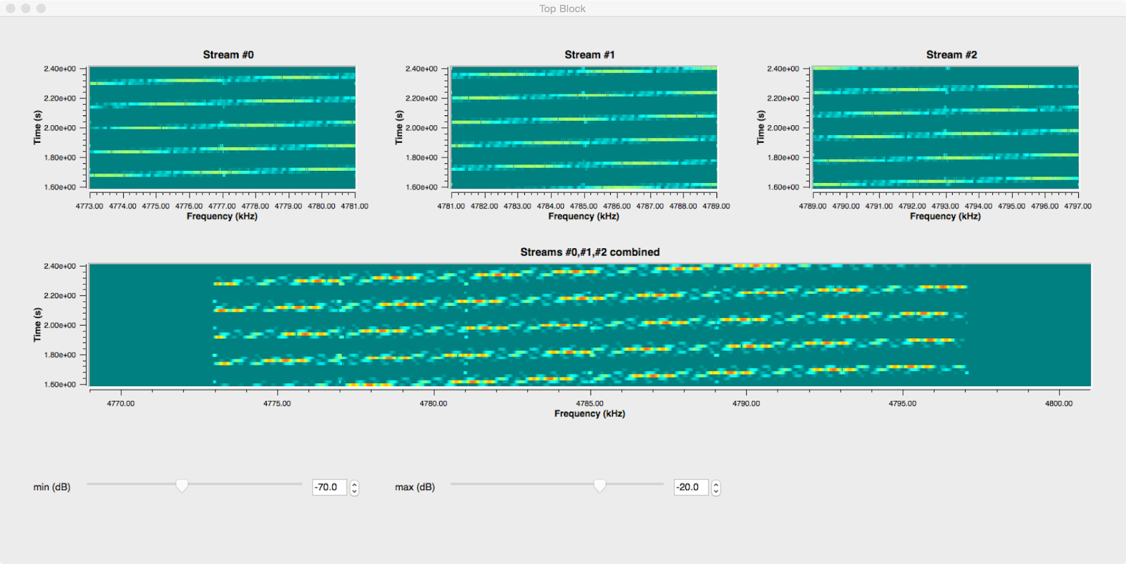
KiwiSDR IQ data streams with >20.25 kHz bandwidth (2)

This is a follow-up on the last blog post. Since then a compensation for the roll-off of the CIC filters in the KiwiSDR FPGA has been implemented in v2.162.

The plot below shows the correction w.r.t. normalized frequency for the 12kHz (20.25kHz) modes in blue (magenta). It is interesting that the main component is in both cases sinc(f)^-5 and that the softening of the correction near f=0.5 can be modeled by an exponential function.

KiwiSDR CIC filter compensation

Another improvement w.r.t. before is to use ±4kHz out of the ±6kHz IQ bandwidth in order to avoid alias images from frequencies below and from above, so the GNURadio flow graph looks now like this:

GNURadio flow graph

This flow graph and the code for the KiwiSDR IQ wav file sources and for the stream align block can be found on GitHub (gr-kiwisdr).

In order to verify that the combination of three IQ data streams@8kHz each to an IQ datastream @32kHz does indeed work, two signals were recorded and processed with the above flow graph:

1.  OTHR signal from Cyprus
   
   

   

   Cyprus OTHR on 14370 kHz @IS0KYB

   As is well-known this signal has a bandwidth of 20kHz and uses a FMCW waveform repeating each 0.02 seconds. When plotting the instantaneous frequency vs. time the FMCW sweeps can be see to be perfectly continuous, i.e., both the alignment of the IQ data streams and the PFB synchronizer work as expected.

   

   Cyprus OTHR on 14370 kHz @IS0KYB

   
   
2. CODAR WCNA
   
   The two plots below show a local CODAR signal recorded on a KiwiSDR in Newport, OR. Also in this case the frequency sweeps can be nicely seen. However it is not clear if the second component in the instantaneous frequency having negative slope is due to interference or due to aliasing in the KiwiSDR downconversion processing.
   
   

   

   Local CODAR signal on 4875 kHz @Newport, OR

   

   Local CODAR signal on 4875 kHz @Newport, OR

The IQ streams used above were recorded using kiwirecorder.py with commands similar to the  following:

./kiwirecorder.py -s sibamanna.duckdns.org,sibamanna.duckdns.org,sibamanna.duckdns.org -p 8073 -f 14362,14370,14378 -m iq -g 55 -w -L -4000 -H +4000 --log-level=info --dt-sec=60 --station=IS0KYB

Using an extended Kalman filter for TDoA HF geo-location

In this post the precision of geo-location using TDoA on shortwave is explored using the data shown on this blog before.

The idea is to feed the time series of time differences into an extended Kalman filter (EKF) using two models for the propagation time from the transmitter to the receiver:

1) Simple ray-geometry for oblique propagation in the ionosphere:

• based on arXiv:1104.2248 which uses the Breit and Tuve + Martyn theorems to convert vertical to oblique incidence
• using vertical electron density profiles from the IRI2016 model as an input
• group refractive index: 1/sqrt(1-f_N²/f²), i.e., no magentoionic effects are taken into account
• when integrating over the group refractive index in the vertical direction, analytic integration of 1/sqrt(f(h)) is performed in each height interval in order to avoid the spurious numerical singularity at the reflection point
• spherical coordinates are used (r_E=6371km)

2) Alternatively, great-circle distances on the WGS84 ellipsoid are used:

• geographiclib adapted for octave

All receiver coordinates are assumed to be in WGS84, however in practice it is suspected that there are deviations from the true locations of up to 20 km, as the KiwiSDR positions are provided by the KiwiSDR owners and are not taken from the GPS position solutions used for time synchronization.

The plot below shows the output of the EKF

• implementation in octave following ADA285972
• state = [lat, lon] of the unknown position
• measurements = time differences between pairs of KiwiSDRs
• the measurements covariance matrix (constant) is build from the covariances of time differences (and is set to zero for time differences not sharing a common receiver)
• state covariance matrix = diag(0.01, 0.01)² deg² (constant)
• start covariance = diag(0.1, 0.1)² deg²
• there are about 60 measurements which are run 5 times sequentially through the EKF

Extended Kalman Filter (EKF) output; note that the range of the x(y) axis corresponds to approximately 17(67)km.

The simple ionosphere propagation model improves the match to the known position but there is still a remaining bias of about 30km North, 4km West. Clearly, more studies are needed in order to find out if this improvement is by chance or real.

De-chirping applied to a HF over the horizon radar signal (2)

This is a follow up to this blog post. Again the signals of the OTHR in Cyprus were analyzed using GPS time-stamped IQ samples from several KiwiSDRs.

In this case the OTHR signal was found between 13965 and 13985 kHz. The slope of the FMCW signal is μ=1MHz/s, and there are 50 sweeps per second. This results in a bandwidth of about 20kHz.

As is well known, the frequencies Δf of the spectrum of the de-chirped signal correspond to time delays τ=-Δf/μ in the case of a stationary target.

• for this one has to multiply the received signal with the original waveform
• tuning offsets w.r.t. center frequency of the OTHR signal correspond to a time delay of the original waveform
• when Δf is positive the delay corresponds to the frequency Δf-f_s (f_s is the sampling frequency), i.e. the ranges wrap around the x-axis.

Applying a 2nd Fourier transform to the time direction of time vs. Δf data one obtains the Doppler frequency f_d vs. Δf where f_d = v•λ/2 (for velocity v and wavelength λ). Here one has to be careful to adjust the phases in each bin to correct for the fact that the sampling times are not exactly aligned to multiples of 0.02 seconds.

Plots for 5 KiwiSDR are shown below. The splitting of the ionospheric reflection is most likely due to O- and X-mode propagation in the F layer.

13975 kHz 20180105T1114Z @CS5SEL; the band at f_d=0 is caused by an interference

13975 kHz 20180105T1114Z @DF0KL

13975 kHz 20180105T1114Z @G8JNJ

13975 kHz 20180105T1114Z @Izhvesk

13975 kHz 20180105T1114Z @Julisdalen

Thanks to all KiwiSDR owners who make their receivers available and do connect a GPS antenna.

De-chirping applied to a HF over the horizon radar signal

Here is another look at the HF OTHR signal from Cyprus already mentioned in this blog post.

This OTHR signal is (at least to 1st order) FMCW modulated (period 0.02 sec, bandwidth 20kHz), as can be seen in the FM demodulated phase which follows a sawtooth pattern with period 0.02 sec.

Although the bandwidth of the KiwiSDR IQ data stream is smaller than the bandwidth of the OTHR signal it turns out that de-chirping can be done: using KiwiSDR GPS time-stamps t, de-chirping can be implemented by multiplying the IQ samples by exp(-2i*pi*f(t)) with f=@(x) 0.5*1e6*(mod(x,0.02)-0.01).**2-50;  (this is octave notation)

The de-chirped signal looks like in the bottom panel below and is flat as expected:

OTHR FM demodulated phase; bottom: de-chirped

The relative range (which includes a contribution from the doppler effect, see, e.g., here) is then obtained by performing a FFT transformation on the de-chirped signal in each 0.02 sec period (~240 samples):

OTHR de-chirped spectrum vs. time

• There is a main reflection in the ionosphere which has an interesting, time-varying structure to the left of it, i.e., towards smaller ranges
• In the light blue regions there is a kind of digital pattern visible; this might be due to the signal processing and limited bandwidth of the KiwiSDR but it could also be caused by some additional modulation of the radar signal

TDoA measurements using GPS time-stamped IQ samples from KiwiSDRs (7)

14370 kHz OTHR 20171211T1040

The autocorrelation function has peaks at multiples of 0.02 seconds: (as is well known)

14370 kHz OTHR autocorrelation

The pulse shapes and the FM demodulated phases are shown below w.r.t. GPS seconds mod 0.02 seconds. Of the full bandwidth of this signal is 20kHz the KiwiSDRs sample 12 kHz. Therefore only part of the chirp signal is seen:

14370 kHz OTHR pulse shape and FM demodulated phase

Correcting for the sample rate the chirpyness becomes 12001*83.326 = 1e6, i.e., one sweep covers 20 kHz.

In the time differences different paths of propagation can be seen; it looks like the ionosphere at this time was quite patchy:

TDoA 14370 kHz

The TDoA location is consistent with the known position of the transmitter:

TDoA maps 14370 kHz

HF over the horizon radar (OTHR)

Here are some notes about an OTHR radar signal (likely the one described  on page 28 here http://www.iarums-r1.org/iarums/radar-2013.pdf) which is audible every evening/night in most of Europe.

Note that there is a bias due to the fact that the KiwiSDR bandwidth (12 kHz) is less than the bandwidth of this radar signal (40-50 kHz)

This is how the autocorrelation looks like:

Autocorrelation

Autocorrelation zoom

• fundamental period: dt = (11573.3 ± 0.2) μs
• the autocorrelation function shows peaks at multiples of dt, 4×dt, and 150×dt

Using GPS time-stamped IQ samples each pulse can be plotted on top of the other pulses:

OTHR pulses

There is a discrete structure in the pulses: pulses with pulse number mod 4 = 0,1,2,3 look more similar:

OTHR pulses - pulse number mod 4