KiwiSDR GNSS position solutions using an extended Kalman filter

This is an update to this blog post, see also https://github.com/jks-prv/Beagle_SDR_GPS/issues/147. References for using Kalman filters for GNSS positioning are, e.g., DST-Group-TR-3260.pdf and these proceedings from ION GPSGNSS 2003.

The plots below show time series of variations in ECEF X,Y,Z coordinates, the oscillator correction, and the number of available satellites.

SPP - single point position; EFK - extended Kalman filter

The process noise covariances are set to 5e-5 for the X,Y,Z coordinates (KiwiSDRs are not expected to move) and the covariances for the time and the oscillator correction are build from Allan variance parameters as described in a497248. It would be interesting to measure the Allan variance of the used oscillator.

The advantages of using an extended Kalman filter include:

• Once a position solution has been obtained, the Kalman filter can be updated with fewer than four satellites: this will improve the availability of those KiwiSDRs with poor GNSS reception for TDoA work.
• The residuals per link in the Kalman filter update are used to exclude satellites with bad time measurements.
• Large deviations from the nominal position due to bad satellite geometries are avoided.

New version of TDoA code available

A version of the 1st idea mentioned in the last blog post is now implemented in the latest version of the TDoA code and thanks to John it is available as an option in the KiwiSDR TDoA service.

The changes in the new TDoA algorithm are the following:

(1) Sanity checks on the recorded IQ wav files

Instead of aborting processing when a single file is found to be bad, stations are now excluded. If more than 1 good station is left, the processing proceeds without the excluded stations. The following checks are performed:

• check for recent GNSS position fixes
• validity check on then GNSS timestamps
• check if |IQ|!=0
• check if the overlap of all wav files is long enough (>10 sec)

(2) Finding clusters in the cross-correlation peaks

For a given pair of stations, peaks in the cross-correlations are found as before. Then these peaks are assembles into up to four clusters using an adaptive clusterization algorithm. It starts by assuming that there are four clusters. If the four clusters are not valid, the algorithm starts again, this time assuming that there are three clusters. When all clusters are valid the algorithm terminates.

The used clusterization algorithm is iterative:

• It starts by assuming that there are N clusters and puts N+1 boundaries b_i at equidistant places between the minimum and maximum time of the cross correlation peaks.
• Then it recomputes the boundaries as follows: Let t_i,i+1 be the average of the mean of the cross correlation peaks between b_i and b_i+1. The boundaries are iteratively updated as b_i=(t_i-1,i+t_i,i+1)/2 until they become constant.
• A cluster is called valid if the distribution of entries in it is not compatible with a random distribution.
• If all clusters are valid or if there is only one cluster (N=1) then the clusterization algorithm terminates.

(3) Selection of those clusters which optimally fulfill the consistency equations

• If there are three stations, cross-correlation times of the same signal fulfill (12)-(13)-(23)=0.
• When there are four stations, there are more of these consistency equations, e.g., (12)-(14)-(24)=0, (23)-(24)-(34)=0 etc.
• For all combinations of clusters all consistency equation are evaluated. Each equation provides the deviation from 0 in terms of number of sigmas (nsigma) using the mean and RMS of the clusters.
• In the end the combination of clusters is selected which for all consistency equations results in the smallest nsigma
• If the nsigma value in any given equation is greater than 3, stations are iteratively excluded until 3 stations are left. The combination of excluded stations which brings max(nsigma) below 3 is not used later on for making the TDoA maps.

New ideas for TDoA multi-lateration

(1) Finding the common propagation mode

Let's consider the case of three receivers receiving the same signal.

• Each receiver receives the signal at times t₁, t₂, t₃.
• The cross-correlations produce time differences Δt_1,2, Δt_1,3, Δt_2,3.
• Trivially, Δt_1,2 = Δt_1,3 - Δt_2,3 (and cyclically) (*)

This situation is illustrated in the plot below.

Common propagation mode

As a second step let's consider the situation when one of the three receivers receives the common signal via two propagation paths, and the cross-correlations to the signals received at the two other receivers have approximately the same magnitude.

Currently the TDoA software performs for each cross-correlation a clustering algorithm, and in the situation shown in the plot below it may well be that the following time differences are obtained: Δt_1,2 = -50, Δt_1,3 = -100, Δt_2,3 = -140. Note that these do not fulfill the identity (*).

Two propagation modes for one receiver

As a consequence, a trivial stage of pre-processing is given by selecting those cross-correlation peaks which are consistent according to (*).

Update 9/22/2018

(2) Using constraints (number of degrees of freedom)

Now let us count the number of degrees of freedom for the case of N receivers receiving the same signal: there are

• 2 unknowns, (lat,lon), for the most likely position
• N unknown virtual heights of which only (N-1) are observable in the time differences (adding a common time offset does not change Δt_i,j)
• N(N-1)/2 hyperbolæ (=constraints)

Note that instead of virtual heights we might as well add time offsets δt_j  to the time differences, Δt_i,j+δt_j, j≠1, and in this way become agnostic w.r.t. the specifics of ionospheric propagation.

As a summary there are N+1 unknowns and N(N-1)/2 constraints:

#receivers	#unknowns	#constraints	#constraints-#unknowns
3	2(pos)+2(δtj, j≠1)	3 hyperbolæ	-1
4	2(pos)+3(δtj, j≠1)	6 hyperbolæ	1
N	2(pos)+(N-1)(δtj, j≠1)	N(N-1)/2 hyperbolæ	N(N-1)/2-N-1

So for 3 receivers there is a 1-dimensional family of solutions while for N≥4 receivers the system of equations is overdetermined.  This sounds good enough to make me suspicious if it is indeed true.

---

It will be interesting to try these ideas on real data obtained from KiwiSDRs. If anyone spots an error in the logic above please do let me know.

---

When using N stations there are N-1 independent measurements contained in the time differences δt_ij, j>i. Two of these are needed to determine the likely position, so N-3 out of the N-1 δt_i, i≠1, can be found:

#receivers	#unknowns	#measurements	#fixed/total δtj
3	2(pos)+2(δtj, j≠1)	2 time differences	0/2
4	2(pos)+3(δtj, j≠1)	3 time differences	1/3
5	2(pos)+4(δtj, j≠1)	4 time differences	2/4
6	2(pos)+5(δtj, j≠1)	5 time differences	3/5
N	2(pos)+(N-1)(δtj, j≠1)	(N-1) time differences	(N-3)/(N-1)

TDoA SuperDARN/Finland

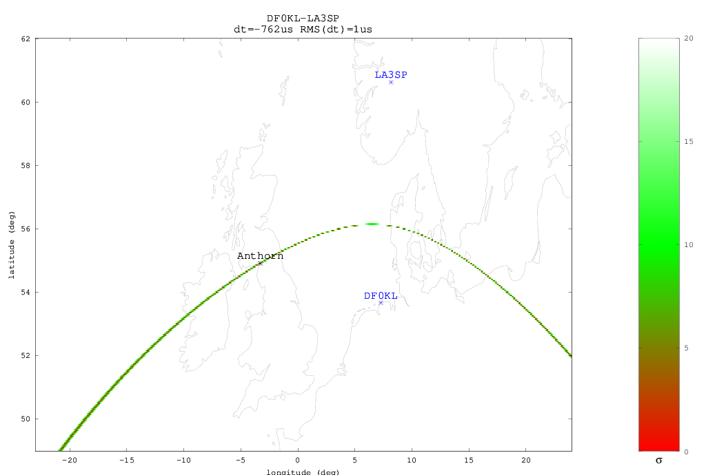
Today signals from the SuperDARN radar in Finland were active around 12375 kHz and the most likely position matches quite well with the known CUTLASS radar position near Hankasalmi.

TDoA maps

TDoA cross correlations

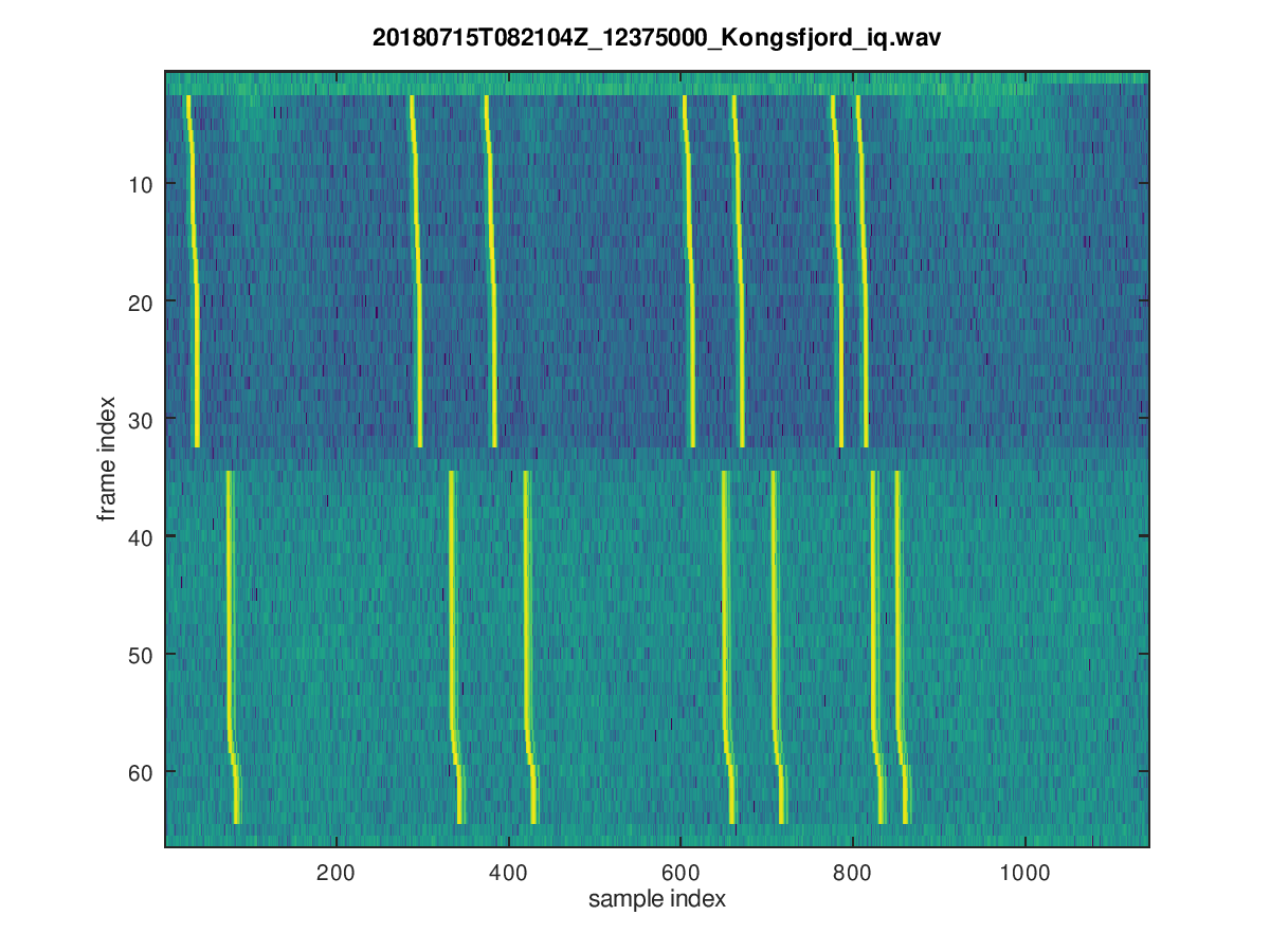
There are pulse trains spaced by integer multiples of 2400 μsec (0,9,12,20,22,26,27), as descibed here:

SuperDARN pulse train

30 of these pulse trains are repeated, approximately each 95.3 msec, then there is a gap of two frames and some delay, and then the next 30 pulse trains follow:

SuperDARN pulse frames

The transmissions seem to repeat each minute with a small gap at the end of the minute.

Another way to verify the used pulse sequence is to compute the autocorrelation of each line of the plot above. All differences between all combinations of the individual pulses show up as peaks in the autocorrelation:

frame number vs. autocorrelation lag

KiwiSDR TDoA (LORAN)

Below is an example of using the new KiwiSDR TDoA extension on LORAN signals, see

• TDoA extension notes
• GitHub repository
• RTL-SDR.com article2 article1

The bias on the most likely position is quite small. Note that despite the fact than one sample at 12kHz is 83.3μs long, the RMS values of the cross correlations are ≤ 6μs. This is because the peaks in the cross correlations are fitted with a 2nd order polynomial.

Fig 1

Fig 2

Fig 3

Fig 4

Fig 5

Fig 6

Fig 7

Propagation delay maps based on IRI2016 electron density profiles

In order to understand better the propagation delay maps used for this blog post, the animation below was created. References for the used method are arXiv:1104.2248 and this well-known book.

Up to 2-hop propagation is considered. In case there is more than one mode of propagation, the smallest non-ground-wave propagation delay is shown in the maps. If there is no ionospheric reflection, the ground-wave delay is shown.

• hop=0: no ionospheric reflection -> ground-wave propagation
• hop=1: one reflection
• hop=2: two reflections 

Propagation delays based on IRI2016 electron density profiles

Propagation delays based on IRI2016 electron density profiles

KiwiSDR TDoA extension

KiwiSDR v1.196 includes a KiwiSDR extension (based on https://github.com/hcab14/TDoA)

Note that ionospheric delays are not taken into account, so depending on the geometry of receivers and the target the TDoA maps will be biased.

Many thanks to John Seamons, ZL/KF6VO.

In parallel I am working on a real-time version of TDoA using python/matplotlib/cartopy.